Lights

Prerequisites

This mini-project draws on materials from:

• Shapes and Colors
• Variables
• Maths
• Classes
• Interactions
• Animations
• Noise
• Sine & Cosine
• Trigonometry and Vectors

Point Sources

In this mini-project we are going to use what we learned about vectors and trigonometry to see how to implement some simple light effects.

This is usually done in a slightly different way in video games, large 3D scenes and virtual environments, but some of the logic is similar and trigonometry is always involved.

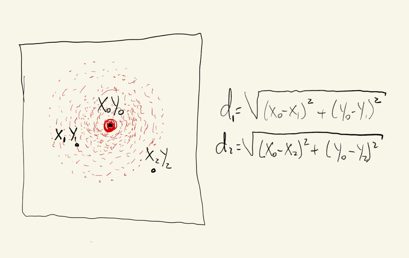
Let’s start with a simple example of a point source, placed in the center of our canvas, that radiates light equally in all directions. Pixels closer to the center will be brighter and pixels further away will be darker.

Our initial intuition might be to code something that iterates over pixels starting in the center of the canvas, coloring in pixels as it moves towards the edges. This could work, but because we want our solution to be generic and eventually work with multiple light sources, it’s actually more efficient and easier to code if we just iterate over the entire canvas and select colors based on distances from the light source.

Since calculating colors for every single pixel is a bit too much work for most browsers, let’s use a parameter to define a grid.

For every point in our grid, we’ll calculate its distance from the center and use map() to pick a color that scales linearly with this distance. Points in the center, with a distance close to \(0\) will have light values close to \(255\), and points that are far from the center will have a color value of \(0\).

This works. We get a nice soft glow effect that almost makes our light source look like a sphere.

We can already see the potential for reorganizing this code using variables for a couple of its parameters, like position, maximum distance, color, etc.

We’ll use fixed values for position and magnitude (how far the light extends), but let’s use a color that’s not white.

We’ll use map() to scale the distance between each pixel and our light’s center to be a value between \(0\) and \(1\). We can pass a sixth argument to the map() function to tell it to clamp the return value so it’s guarantee to be within our output range. In our case, we want any values beyond the mMag value to just be considered a \(1\).

Once we have a value that maps distances from our light source to values between \(0\) and \(1\), we can use the lerpColor() function to pick color values that go from our full color to \(0\).

Change mColor, mMag and mPos above ☝️ to see how each of them affects the output.

Let’s continue to refactor this code and put our logic inside a class, so we can prepare to have multiple light sources.

Our class will have a constructor for setting initial light parameters, a set() function for setting its position, and a get() function to return the color value at a given location on our canvas.

We can even attach our light to the mouse position.

There are a couple of things we can experiment with.

Easing

First, different radiance functions.

Our light has a linear brightness function right now, meaning that the color of any given pixel is directly proportional to its distance from the light. That’s not really how lights work. Instead of map() we can use a different easing function to get a value between \(0\) and \(1\) that has a more complex relationship with distance.

We’ll continue to use map() to scale the distance value from \([0, mag]\) to \([0, 1]\), but then we’ll use some nonlinear functions to change how quickly this relative distance value between \([0, 1]\) goes from light to dark.

EaseIn functions change more abruptly towards the end of their range, so they’ll create light sources that have a brighter center. EaseOut functions change more quickly in the beginning, so they’ll fade to black sooner.

And since now we have multiple light sources, we’ll use a function to add their individual contributions to the overall pixel color:

function addColors(c0, c1) {
  return color(red(c0) + red(c1), green(c0) + green(c1), blue(c0) + blue(c1));
}

The second thing we could do is add a bit of a glow animation to our light.

We can use the sin() function to create a glow parameter with a period of \(1500\) milliseconds and add it to the mag value of our light to make it seem like it’s pulsating:

let glow = sin(TWO_PI / 1500 * millis());

Neat ! 🍸

Let’s move the logic for adding two colors inside our light class. We’ll add an optional parameter to our get() function, that, when present, gets added to the color being returned.

It’s easier to test and see how colors get added now:

Just one last thing, let’s have some lights with movement.

We’ll use polar coordinates and noise() to create some circular paths for our lights, and see how they interact.